7 min to read
California Housing Price Prediction

Let’s first have a quick look at the dataset:
| longitude | latitude | median_house_age | total_rooms | total_bedrooms | population | households | median_income | median_house_value | ocean_proximity |
|---|---|---|---|---|---|---|---|---|---|
| -122.23 | 37.88 | 41.0 | 880.0 | 129.0 | 322.0 | 126.0 | 8.3252 | 452600.0 | NEAR BAY |
| -122.22 | 37.86 | 21.0 | 7099.0 | 1106.0 | 2401.0 | 1138.0 | 8.3014 | 358500.0 | NEAR BAY |
| -122.24 | 37.85 | 52.0 | 1467.0 | 190.0 | 496.0 | 177.0 | 7.2574 | 352100.0 | NEAR BAY |
| -122.25 | 37.85 | 52.0 | 1274.0 | 235.0 | 558.0 | 219.0 | 5.6431 | 341300.0 | NEAR BAY |
| -122.25 | 37.85 | 52.0 | 1627.0 | 280.0 | 565.0 | 259.0 | 3.8462 | 342200.0 | NEAR BAY |
Let’s also look at the fields in the dataset, their types and the amount of examples present in each attribute of the dataset
<class 'pandas.core.frame.DataFrame'>
RangeIndex: 20640 entries, 0 to 20639
Data columns (total 10 columns):
longitude             20640 non-null float64
latitude              20640 non-null float64
housing_median_age    20640 non-null float64
total_rooms           20640 non-null float64
total_bedrooms        20433 non-null float64
population            20640 non-null float64
households            20640 non-null float64
median_income         20640 non-null float64
median_house_value    20640 non-null float64
ocean_proximity       20640 non-null object
dtypes: float64(9), object(1)
memory usage: 1.6+ MB
There are 20640 instances in the dataset but the ‘total_bedrooms’ attribute has only 20433 non-null values, meaning 207 districts are missing this feature. All numerical values except the ‘ocean_proximity’ field. Its type is object, so it could hold ay kind of python object, but since the data is loaded from a CSV file, we know it must be a text attribute.
Let’s see what values or categories exists in ‘ocean_proximity’ column and how many instances(i.e. districts in this case) belong to each category:
<1H OCEAN     9136
INLAND        6551
NEAR OCEAN    2658
NEAR BAY      2290
ISLAND           5
Name: ocean_proximity, dtype: int64
Lets also have a look at the summary of all numerical attributes:
| longitude | latitude | housing_median_age | total_rooms | total_bedrooms | population | households | median_income | median_house_value | |
|---|---|---|---|---|---|---|---|---|---|
| count | 20640.000000 | 20640.000000 | 20640.000000 | 20640.000000 | 20433.000000 | 20640.000000 | 20640.000000 | 20640.000000 | 20640.000000 |
| mean | -119.569704 | 35.631861 | 28.639486 | 2635.763081 | 537.870553 | 1425.476744 | 499.539680 | 3.870671 | 206855.816909 |
| std | 2.003532 | 2.135952 | 12.585558 | 2181.615252 | 421.385070 | 1132.462122 | 382.329753 | 1.899822 | 115395.615874 |
| min | -124.350000 | 32.540000 | 1.000000 | 2.000000 | 1.000000 | 3.000000 | 1.000000 | 0.499900 | 14999.000000 |
| 25% | -121.800000 | 33.930000 | 18.000000 | 1447.750000 | 296.000000 | 787.000000 | 280.000000 | 2.563400 | 119600.000000 |
| 50% | -118.490000 | 34.260000 | 29.000000 | 2127.000000 | 435.000000 | 1166.000000 | 409.000000 | 3.534800 | 179700.000000 |
| 75% | -118.010000 | 37.710000 | 37.000000 | 3148.000000 | 647.000000 | 1725.000000 | 605.000000 | 4.743250 | 264725.000000 |
| max | -114.310000 | 41.950000 | 52.000000 | 39320.000000 | 6445.000000 | 35682.000000 | 6082.000000 | 15.000100 | 500001.000000 |
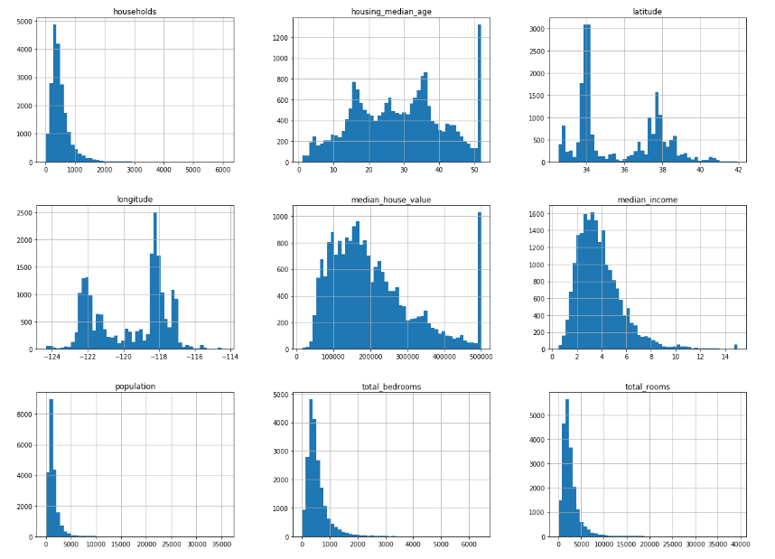
A quick look at the distribution of all numerical attributes states that the median_income is a very important attribute in predicting the median_house_value (which is our label). We therefore, need to ensure that test set is representative of the various categories of incomes in the whole dataset. Since the median income is a continuous numerical attribute, we first need to create an income category attribute. Its important to have a significant number of instances in the dataset for each stratum, or else the estimate of the stratum’s importance may be biased. This means that we can’t afford to have too many strata, and each strata should be large enough.
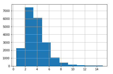
creating an income category attribute by dividing the median_income by 1.5 (just to limit the number of income categories), and rounding up using ceil function (to have proper discrete categories), and then merging all the categories greater than 5 into category 5.
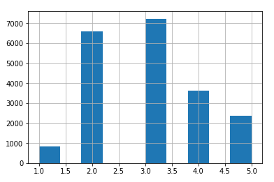
Now we’re ready to do the split the dataset into training and testing data, but first lets look at the proportions of instances w.r.t. our true-label across different approaches fo splitting:
| Overall | Random | Stratified | Rand. %error | Strat. %error | |
|---|---|---|---|---|---|
| 1.0 | 0.039826 | 0.040213 | 0.039729 | 0.973236 | -0.243309 |
| 2.0 | 0.318847 | 0.324370 | 0.318798 | 1.732260 | -0.015195 |
| 3.0 | 0.350581 | 0.358527 | 0.350533 | 2.266446 | -0.013820 |
| 4.0 | 0.176308 | 0.167393 | 0.176357 | -5.056334 | 0.027480 |
| 5.0 | 0.114438 | 0.109496 | 0.114583 | -4.318374 | 0.127011 |
As can be seen, the test set generated using stratified sampling has income category proportions almost identical to those in the full dataset, whereas the test set generated using random sampling is quite skewed.
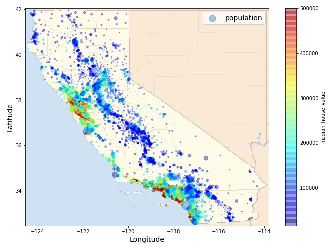
Since there is geographical coordinates present in the data, let’s have a look at the population and median_house_values of the house listings in California,
So far, we’ve framed the problem, got the data and explored it, sampled a training set and a test set, wrote a trasformation pipeline to clean up and prepare the data for Machine Learning algorithms automatically. Now to select and train a ML model.
Trying out Linear Regression model,
LinearRegression(copy_X=True, fit_intercept=True, n_jobs=1, normalize=False)

Predictions on some random data points: [210644.60459286, 317768.80697211, 210956.43331178,  59218.98886849, 189747.55849879]
comparing against the actual values these random data points: [286600.0, 340600.0, 196900.0, 46300.0, 254500.0]
not exactly accurate! Let’s measure the regression model’s RMSE on the whole training set 68628.19819848923
most district’s median_housing_values range between 120,000 (i.e. 25th quadrant) and 265,000 (i.e. 75th quadrant), so there’s a typical prediction error of $ 68,628 in the median_housing_values.
A clear case of model underfitting the training data. This means either the features do not provide enough information to make good predictions, or that the model is not powerful enough. The main ways to fix underfitting are to select a more powerful model, to feed the training algorithm with better features, or to reduce the constraints on the model. As this model is not regularized, this rules out the last option.
Decision Tree Regressor model,
DecisionTreeRegressor(criterion='mse', max_depth=None, max_features=None,
           max_leaf_nodes=None, min_impurity_decrease=0.0,
           min_impurity_split=None, min_samples_leaf=1,
           min_samples_split=2, min_weight_fraction_leaf=0.0,
           presort=False, random_state=None, splitter='best')

Mean RMSE after CV: 71005.03244048063
Standard deviation in RMSE after CV: 2626.4754774424796
this is even worse than Linear Regression model! The Decision Tree has a score of approximately 70,960, generally ±2525. Lets compute the scores for the Linear Regression model as well just to be sure.
Mean RMSE after CV: 69052.46136345083
Standard deviation in RMSE after CV: 2731.6740017983425
Its quite clear the Decision Tree model is overfitting so badly that it performs worse than the Linear Regression model.
Random Forest Regressor model,
RandomForestRegressor(bootstrap=True, criterion='mse', max_depth=None,
           max_features='auto', max_leaf_nodes=None,
           min_impurity_decrease=0.0, min_impurity_split=None,
           min_samples_leaf=1, min_samples_split=2,
           min_weight_fraction_leaf=0.0, n_estimators=10, n_jobs=1,
           oob_score=False, random_state=42, verbose=0, warm_start=False)

Mean RMSE after CV: 52564.19025244012
Standard deviation in RMSE after CV: 2301.873803919754
this is much better! Random Forest looks very promising. However the score on the training set is still much lower than on the validation sets, meaning that the model is still overfitting the training set. So fine-tuning the hyperparameters of the model now.
RandomizedSearchCV(cv=5, error_score='raise',
          estimator=RandomForestRegressor(bootstrap=True, criterion='mse', max_depth=None,
           max_features='auto', max_leaf_nodes=None,
           min_impurity_decrease=0.0, min_impurity_split=None,
           min_samples_leaf=1, min_samples_split=2,
           min_weight_fraction_leaf=0.0, n_estimators=10, n_jobs=1,
           oob_score=False, random_state=42, verbose=0, warm_start=False),
          fit_params=None, iid=True, n_iter=10, n_jobs=1,
          param_distributions={'n_estimators': <scipy.stats._distn_infrastructure.rv_frozen object at 0x000000B944F3C748>, 'max_features': <scipy.stats._distn_infrastructure.rv_frozen object at 0x000000B944F3C518>},
          pre_dispatch='2*n_jobs', random_state=42, refit=True,
          return_train_score='warn', scoring='neg_mean_squared_error',
          verbose=0)

Final RMSE after feature importance: 48304.90942918668
Saving the model persistence with joblib,
from sklearn.externals import joblib
joblib.dump(my_model, "my_model.pkl")
Check out the whole exploratory data analysis and predictive model building as notebook here.
If you liked this project, please consider buying me a coffee

Comments